Madeline A. Ward published a paper on methods for detecting seasonal influenza epidemics using school absenteeism data. The premise is that there is a school absenteeism surveillance system established in Wellington-Dufferin-Guelph which uses a threshold-based (10% of students absent) approach to raise alarms for school illness outbreaks to implement mitigating measures. Two metrics (FAR and ADD) are proposed in that study that were found to be more accurate.
Based on the work of Madeline, in 2021 Kayla Vanderkruk along with Drs. Deeth and Feng wrote a paper on improved metrics, namely ATQ (alert time quality), that are more accurate and timely than the FAR-selected models. This package is based off Kayla’s work that can be found here. ATQ study assessed alarms on a gradient, where alarms raised incrementally before or after an optimal date were penalized for lack of timeliness.
This ATQ package will allow users to perform simulation studies and evaluate ATQ & FAR based metrics from them. The simulation study will require information from census data for a region such as distribution of number of household members, households with and without children, and age category, etc.
This package is still a work in progress and future considerations include streamlining simulation study workflow and generalizing evaluation of metrics to include real data sets.
You can install the development version of ATQ from Github
#install.packages("devtools")
library(devtools)
install_github("vjoshy/ATQ_Surveillance_Package")The ATQ package includes the following main functions:
catchment_sim()
elementary_pop()
subpop_children()
subpop_noChildren()
simulate_households()
ssir()
compile_epi()
eval_metrics()
plot() and summary()
Additionally, the package implements S3 methods for generic functions:
plot() and summary()
ssir() and eval_metrics()plot() provides visualizations of epidemic simulations
and metric evaluationssummary() offers concise summaries of the simulation
results and metric assessmentsThese functions and methods work together to facilitate comprehensive epidemic simulation and evaluation of detection models
Please see example below:
# Load the ATQ package
library(ATQ)
set.seed(69420)
#Simulate number of elementary schools in each catchment
catch_df <- catchment_sim(16, 5, shape = 4.68, rate = 3.01)
# Simulate elementary school populations for each catchment area
elementary_df <- elementary_pop(catch_df, shape = 5.86, rate = 0.01)
# Simulate households with children
house_children <- subpop_children(elementary_df, n = 2,
prop_parent_couple = 0.7,
prop_children_couple = c(0.3, 0.5, 0.2),
prop_children_lone = c(0.4, 0.4, 0.2),
prop_elem_age = 0.6)
# Simulate households without children
house_nochildren <- subpop_noChildren(house_children, elementary_df,
prop_house_size = c(0.2, 0.3, 0.25, 0.15, 0.1),
prop_house_Children = 0.3)
# Combine household simulations and generate individual-level data
simulation <- simulate_households(house_children, house_nochildren)
# Extract individual-level data
individuals <- simulation$individual_sim
# Simulate epidemic using SSIR (Stochastic Susceptible-Infectious-Recovered) model
epidemic <- ssir(nrow(individuals), T = 300, alpha = 0.298, inf_init = 32, rep = 10)
# Summarize and plot the epidemic simulation results
summary(epidemic)
#> SSIR Epidemic Summary (Multiple Simulations):
#> Number of simulations: 10
#>
#> Average total infected: 41065.5
#> Average total reported cases: 826.9
#> Average peak infected: 3036.4
#>
#> Model parameters:
#> $N
#> [1] 136784
#>
#> $T
#> [1] 300
#>
#> $alpha
#> [1] 0.298
#>
#> $inf_period
#> [1] 4
#>
#> $inf_init
#> [1] 32
#>
#> $report
#> [1] 0.02
#>
#> $lag
#> [1] 7
#>
#> $rep
#> [1] 10
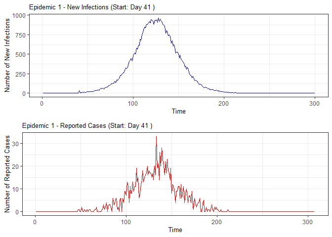
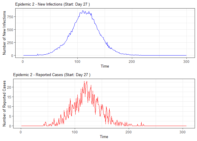
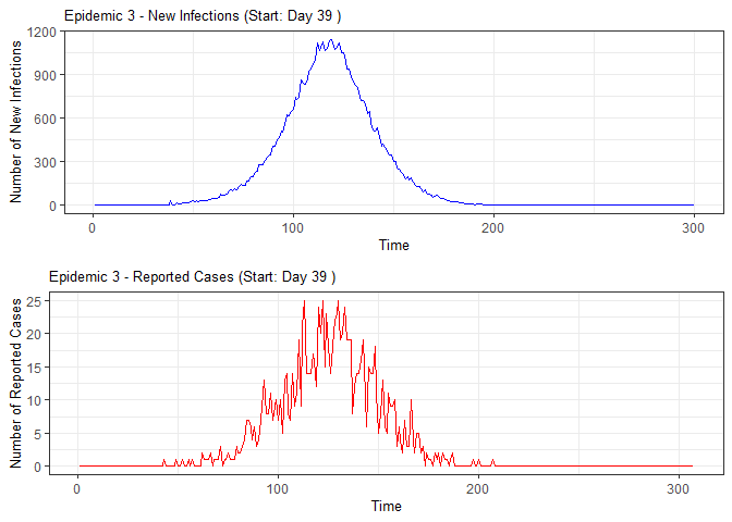
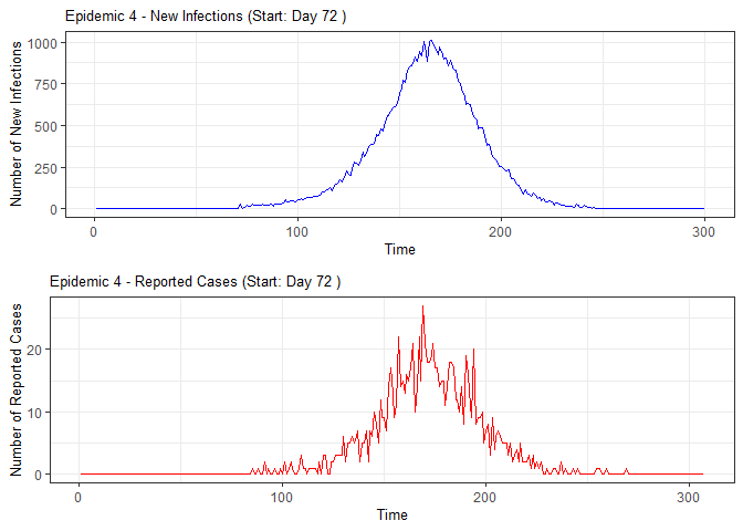
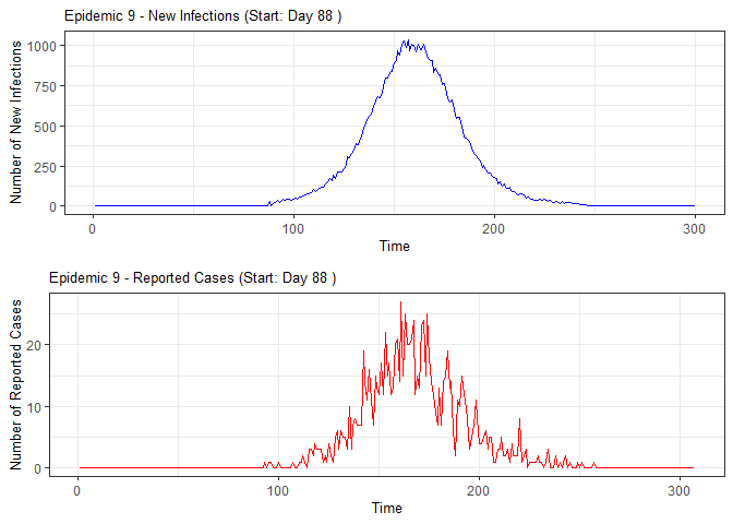
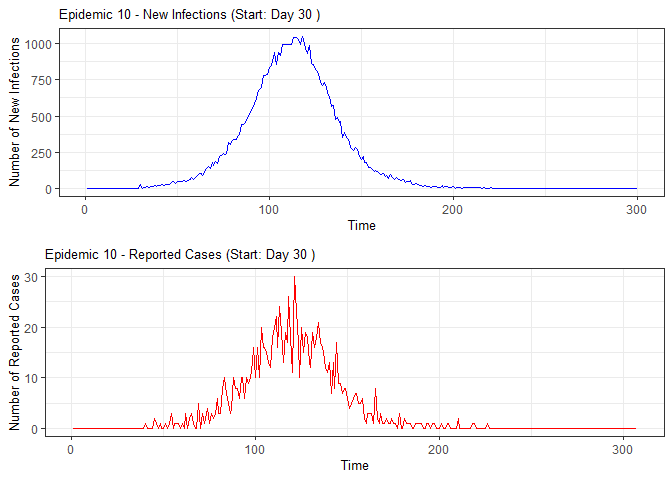
plot(epidemic)
# Compile absenteeism data based on epidemic simulation and individual data
absent_data <- compile_epi(epidemic, individuals)

# Display structure of absenteeism data
dplyr::glimpse(absent_data)
#> Rows: 3,000
#> Columns: 28
#> $ Date        <int> 1, 2, 3, 4, 5, 6, 7, 8, 9, 10, 11, 12, 13, 14, 15, 16, 17,…
#> $ ScYr        <int> 1, 1, 1, 1, 1, 1, 1, 1, 1, 1, 1, 1, 1, 1, 1, 1, 1, 1, 1, 1…
#> $ pct_absent  <dbl> 0.05096603, 0.05190044, 0.05079590, 0.04899765, 0.05083607…
#> $ absent      <dbl> 636, 661, 628, 627, 623, 624, 607, 603, 657, 673, 616, 667…
#> $ absent_sick <dbl> 0, 0, 0, 0, 0, 0, 0, 0, 0, 0, 0, 0, 0, 0, 0, 0, 0, 0, 0, 0…
#> $ new_inf     <dbl> 0, 0, 0, 0, 0, 0, 0, 0, 0, 0, 0, 0, 0, 0, 0, 0, 0, 0, 0, 0…
#> $ lab_conf    <dbl> 0, 0, 0, 0, 0, 0, 0, 0, 0, 0, 0, 0, 0, 0, 0, 0, 0, 0, 0, 0…
#> $ Case        <dbl> 0, 0, 0, 0, 0, 0, 0, 0, 0, 0, 0, 0, 0, 0, 0, 0, 0, 0, 0, 0…
#> $ sinterm     <dbl> 0.01720158, 0.03439806, 0.05158437, 0.06875541, 0.08590610…
#> $ costerm     <dbl> 0.9998520, 0.9994082, 0.9986686, 0.9976335, 0.9963032, 0.9…
#> $ window      <dbl> 0, 0, 0, 0, 0, 0, 0, 0, 0, 0, 0, 0, 0, 0, 0, 0, 0, 0, 0, 0…
#> $ ref_date    <dbl> 0, 0, 0, 0, 0, 0, 0, 0, 0, 0, 0, 0, 0, 0, 0, 0, 0, 0, 0, 0…
#> $ lag0        <dbl> 0.05096603, 0.05190044, 0.05079590, 0.04899765, 0.05083607…
#> $ lag1        <dbl> NA, 0.05096603, 0.05190044, 0.05079590, 0.04899765, 0.0508…
#> $ lag2        <dbl> NA, NA, 0.05096603, 0.05190044, 0.05079590, 0.04899765, 0.…
#> $ lag3        <dbl> NA, NA, NA, 0.05096603, 0.05190044, 0.05079590, 0.04899765…
#> $ lag4        <dbl> NA, NA, NA, NA, 0.05096603, 0.05190044, 0.05079590, 0.0489…
#> $ lag5        <dbl> NA, NA, NA, NA, NA, 0.05096603, 0.05190044, 0.05079590, 0.…
#> $ lag6        <dbl> NA, NA, NA, NA, NA, NA, 0.05096603, 0.05190044, 0.05079590…
#> $ lag7        <dbl> NA, NA, NA, NA, NA, NA, NA, 0.05096603, 0.05190044, 0.0507…
#> $ lag8        <dbl> NA, NA, NA, NA, NA, NA, NA, NA, 0.05096603, 0.05190044, 0.…
#> $ lag9        <dbl> NA, NA, NA, NA, NA, NA, NA, NA, NA, 0.05096603, 0.05190044…
#> $ lag10       <dbl> NA, NA, NA, NA, NA, NA, NA, NA, NA, NA, 0.05096603, 0.0519…
#> $ lag11       <dbl> NA, NA, NA, NA, NA, NA, NA, NA, NA, NA, NA, 0.05096603, 0.…
#> $ lag12       <dbl> NA, NA, NA, NA, NA, NA, NA, NA, NA, NA, NA, NA, 0.05096603…
#> $ lag13       <dbl> NA, NA, NA, NA, NA, NA, NA, NA, NA, NA, NA, NA, NA, 0.0509…
#> $ lag14       <dbl> NA, NA, NA, NA, NA, NA, NA, NA, NA, NA, NA, NA, NA, NA, 0.…
#> $ lag15       <dbl> NA, NA, NA, NA, NA, NA, NA, NA, NA, NA, NA, NA, NA, NA, NA…

# Evaluate alarm metrics for epidemic detection
alarm_metrics <- eval_metrics(absent_data, thres = seq(0.1,0.6,by = 0.05))

# Plot various alarm metrics
plot(alarm_metrics$metrics, "FAR")   # False Alert Rate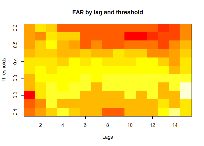
plot(alarm_metrics$metrics, "FATQ") # First Alert Time Quality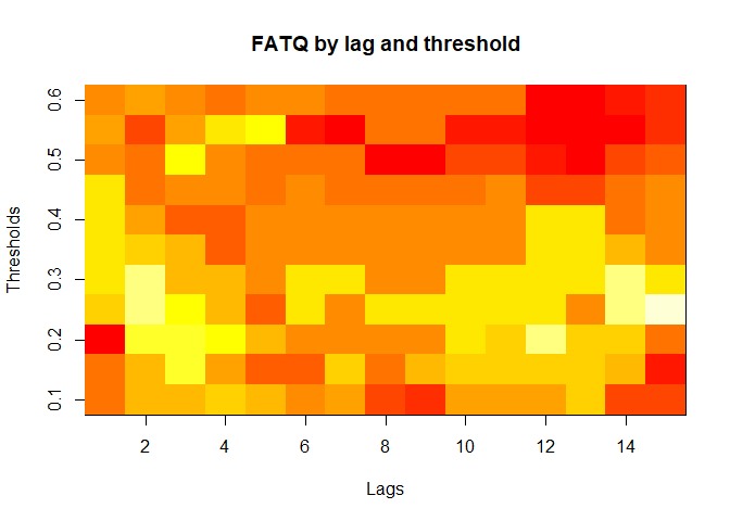
plot(alarm_metrics$metrics, "AATQ") # Average Alert Time Quality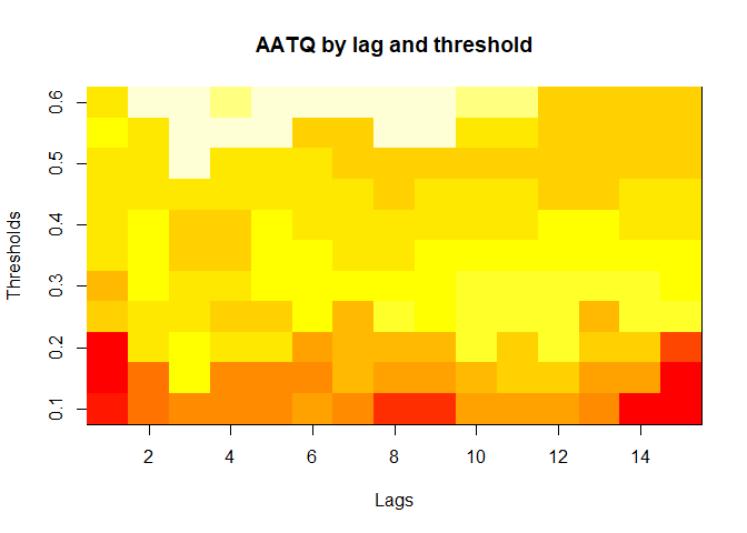
plot(alarm_metrics$metrics, "WAATQ") # Weighted Average Alert Time Quality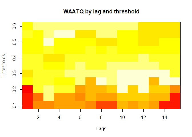
plot(alarm_metrics$metrics, "WFATQ") # Weighted First Alert Time Quality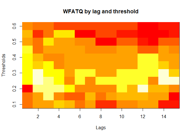
plot(alarm_metrics$metrics, "ADD") # Accumulated Delay Days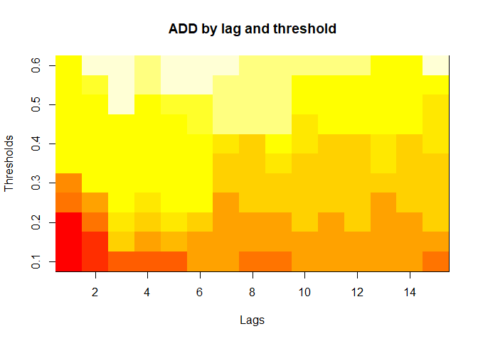
# Summarize alarm metrics
summary(alarm_metrics$results)
#> Alarm Metrics Summary
#> =====================
#>
#> FAR :
#> Mean: 0.5603
#> Variance: 0.0191
#> Best lag: 9
#> Best threshold: 0.1
#> Best value: 0.2111
#>
#> ADD :
#> Mean: 25.831
#> Variance: 75.0129
#> Best lag: 1
#> Best threshold: 0.1
#> Best value: 6.1111
#>
#> AATQ :
#> Mean: 0.542
#> Variance: 0.028
#> Best lag: 2
#> Best threshold: 0.1
#> Best value: 0.1861
#>
#> FATQ :
#> Mean: 0.5451
#> Variance: 0.0228
#> Best lag: 9
#> Best threshold: 0.1
#> Best value: 0.1964
#>
#> WAATQ :
#> Mean: 0.5288
#> Variance: 0.0313
#> Best lag: 1
#> Best threshold: 0.15
#> Best value: 0.1373
#>
#> WFATQ :
#> Mean: 0.5474
#> Variance: 0.0217
#> Best lag: 4
#> Best threshold: 0.1
#> Best value: 0.2516
#>
#> Reference Dates:
#> epidemic_years ref_dates
#> 1 1 53
#> 2 2 64
#> 3 3 43
#> 4 4 61
#> 5 5 45
#> 6 6 49
#> 7 7 40
#> 8 8 48
#> 9 9 61
#> 10 10 79
#>
#> Best Prediction Dates:
#> FAR :
#> [1] NA 50 42 54 45 40 31 NA 55 52
#>
#> ADD :
#> [1] NA 47 NA 43 24 35 31 26 33 6
#>
#> AATQ :
#> [1] NA 47 NA 46 30 36 30 32 37 31
#>
#> FATQ :
#> [1] NA 50 42 54 45 40 31 NA 55 52
#>
#> WAATQ :
#> [1] NA 48 NA 43 24 35 37 26 37 31
#>
#> WFATQ :
#> [1] NA 46 NA 52 33 37 31 41 55 24
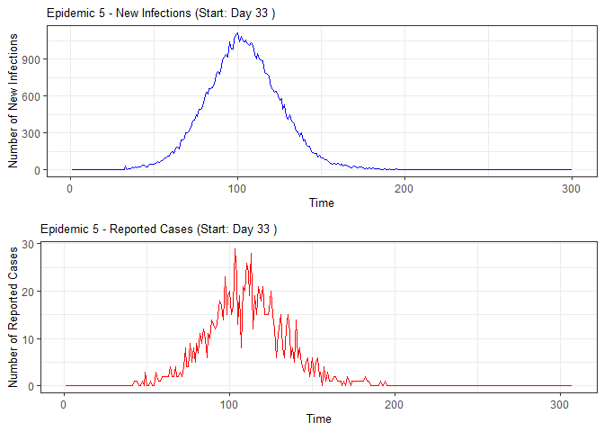
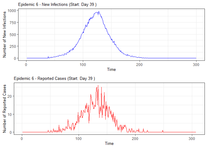
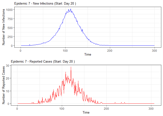
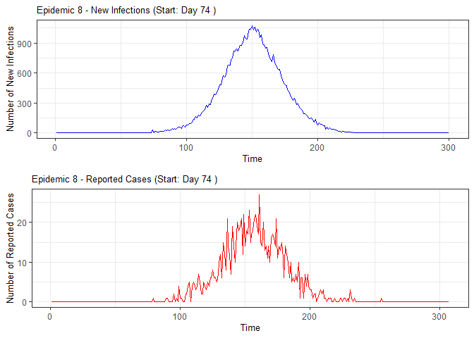
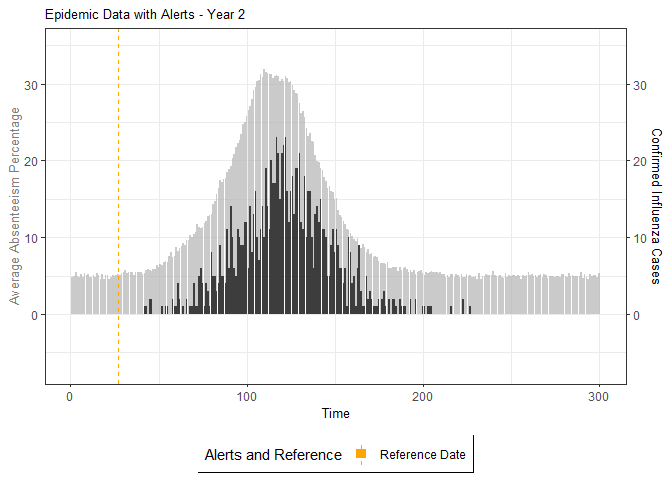
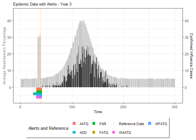
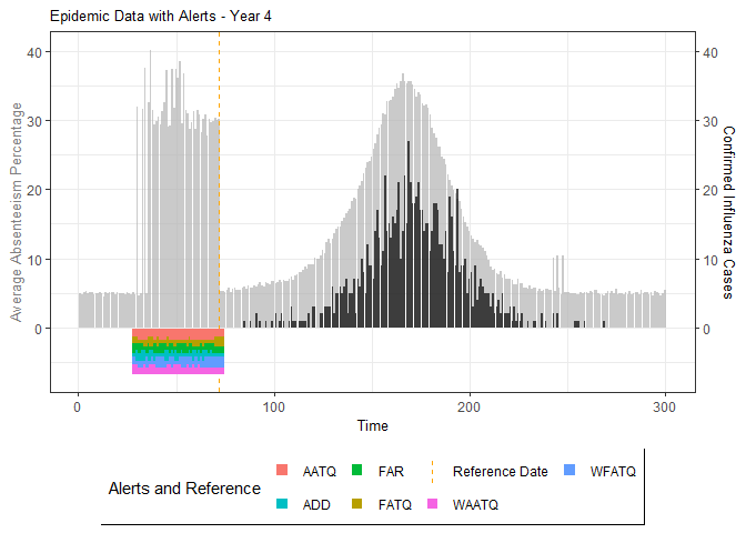
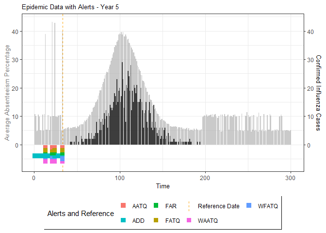
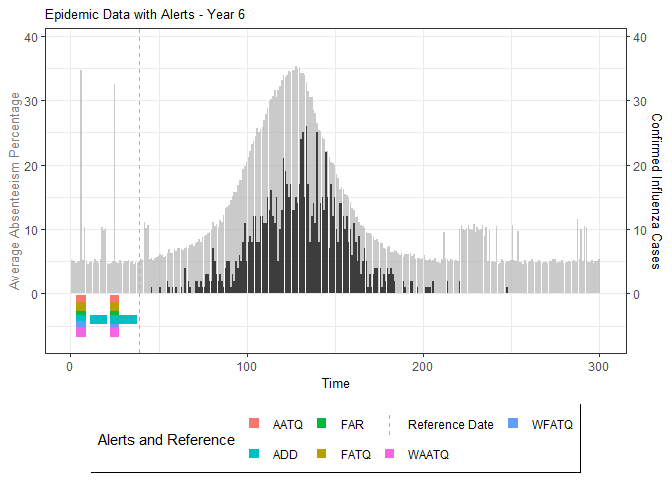
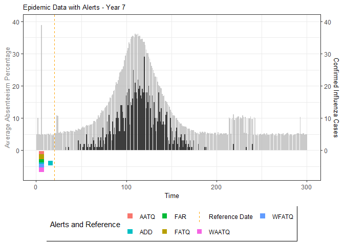
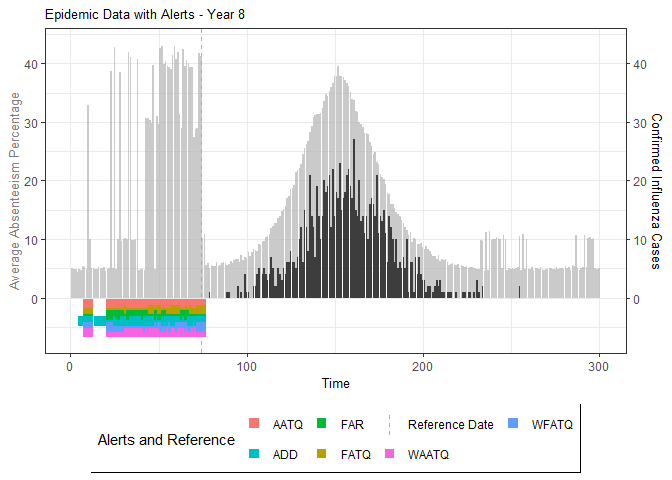
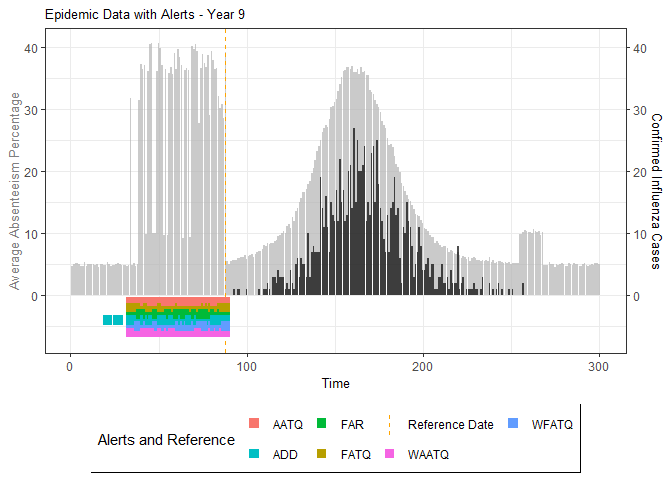
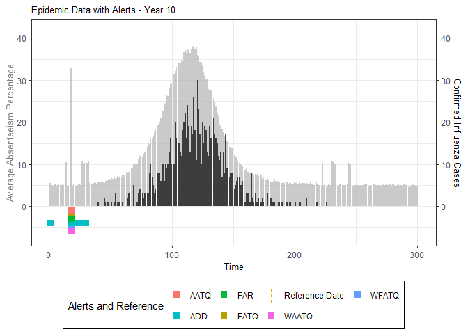
# Generate and display plots for alarm metrics across epidemic years
alarm_plots <- plot(alarm_metrics$plot_data)
for(i in seq_along(alarm_plots)) {
print(alarm_plots[[i]])
}
The final output region_metric will be a list of 6
matrices and 6 data frames. The matrices describe the values of metrics
for respective lag and thresholds.
An optimal lag and threshold value that minimizes each metric is selected and these optimal parameters are used to generate the 6 data frames associated with the metrics. Simulated information like number of lab confirmed cases, number of students absent, etc, are also included in the output.