![]()
![]()
![]()
The goal of spatialising is to perform simulations of binary spatial raster data using the Ising model.
You can install the released version of spatialising from CRAN with:
install.packages("spatialising")You can install the development version of spatialising from GitHub with:
# install.packages("devtools")
devtools::install_github("Nowosad/spatialising")The spatialising package expects raster data with
just two values, -1 and 1. Here, we will use
the r_start.tif file built in the package.
library(spatialising)
library(terra)
r1 = rast(system.file("raster/r_start.tif", package = "spatialising"))
plot(r1)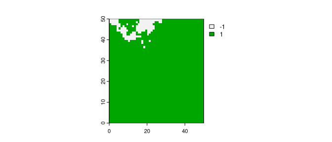
Most of the raster area is covered with the value of 1,
and just about 5% of the area is covered with the value of
-1. The main function in this package is
kinetic_ising(). It accepts the input raster and at least
two additional parameters: B – representing external
pressure and J – representing the strength of the local
autocorrelation tendency. The output is a raster modified based on the
provided parameters.
r2 = kinetic_ising(r1, B = -0.3, J = 0.7)
plot(r2)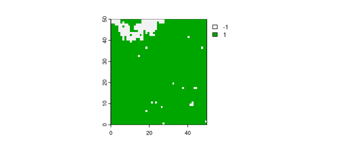
The kinetic_ising() function also has a fourth argument
called updates. By default, it equals to 1,
returning just one raster as the output. However, when given a value
larger than one, it returns many rasters. Each new raster is the next
iteration of the Ising model of the previous one.
ri1 = kinetic_ising(r1, B = -0.3, J = 0.7, updates = 3)
plot(ri1, nr = 1)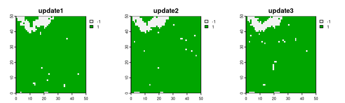
Obtained results depend greatly on the set values of B
and J. In the example above, values of
B = -0.3 and J = 0.7 resulted in expansion of
the yellow category (more -1 values).
On the other hand, values of B = 0.3 and
J = 0.7 give a somewhat opposite result with less cell with
the yellow category:
ri2 = kinetic_ising(r1, B = 0.3, J = 0.7, updates = 3)
plot(ri2, nr = 1)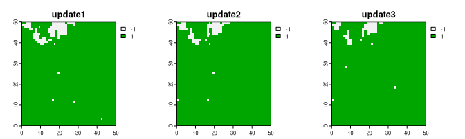
Finally, in the last example, we set values of B = -0.3
and J = 0.4. Note that the result shows much more prominent
data change, with a predominance of the yellow category only after a few
updates.
ri3 = kinetic_ising(r1, B = -0.3, J = 0.4, updates = 3)
plot(ri3, nr = 1)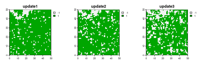
Read the related article:
Contributions to this package are welcome - let us know if you have any suggestions or spotted a bug. The preferred method of contribution is through a GitHub pull request. Feel also free to contact us by creating an issue.